Authors: Moussa Koulako Bala Doumbouya, Dan Jurafsky, Christopher D. Manning
Paper: https://arxiv.org/abs/2506.11035
Once a year, some interesting architecture inevitably appears where they change some fundamental building block. This happened with KAN last year, where they changed the parameterization of the neuron activation function (though it's unclear what the outcome is after a year — many follow-up works seem to have appeared, but KANs haven't displaced anyone anywhere yet). The same is true in this current work, where they change the proximity function from the classic scalar product as in transformers (or cosine similarity, which is roughly the same) to a more sophisticated asymmetric function named after Amos Tversky. Jurafsky and Manning are co-authors (and in KANs, Tegmark was a co-author), so these aren't exactly random people.
Modern deep learning architectures, from CNNs to transformers, are built on a fundamental but often overlooked assumption: similarity between concepts can be measured geometrically using functions like dot product or cosine similarity. While this approach is computationally convenient, cognitive psychology has long known that this geometric model poorly reflects human similarity judgments. As Amos Tversky noted in his landmark 1977 work, human perception of similarity is often asymmetric — we say that a son resembles his father more than the father resembles the son. This asymmetry violates the metric properties inherent in geometric models.
Tversky proposed an alternative: a feature matching model where similarity is a function of common and distinctive features. Despite its psychological plausibility, this model relied on discrete set operations, making it incompatible with the differentiable, gradient-based optimization that underlies modern deep learning. The authors of this paper have elegantly bridged this gap.
The key innovation is a differentiable parameterization of Tversky similarity. The authors propose a dual representation where objects are simultaneously both vectors (as usual, of Rd dimensionality) and feature sets (this is new). A feature (from a given finite set Ω) is considered "present" in an object if the scalar product of the object vector and the feature vector is positive. This construction allows reformulating traditionally discrete intersection and difference operations as differentiable functions.
The Tversky similarity function is defined as:
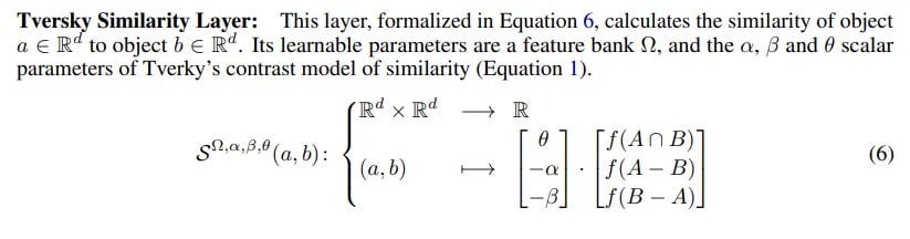
S(a, b) = θf(A ∩ B) − αf(A − B) − βf(B − A), (1)
where A and B are the feature sets of objects a and b, and {θ, α, β} are learnable parameters. In this formula, the first term accounts for common features, the second for distinctive features of object a, and the third for distinctive features of object b.
The following functions are defined for features:
Salience or prominence of features of object A is the sum of positive scalar products for features present in the object. A less salient object (e.g., son) is more similar to a more salient object (father) than vice versa.
Intersection (common features) of objects A and B is defined through function Ψ, which aggregates features present in both objects. They tried min, max, product, mean, gmean, softmin as Ψ.
Difference (features present in the first object but absent in the second) is defined in two ways. The first, ignorematch, only considers features present in A but not in B. The other method, subtractmatch, also considers features present in both objects but more pronounced in A.
Next, Tversky neural networks are defined based on two new building blocks:
Tversky Similarity Layer, analogous to metric similarity functions like dot product or cosine similarity. Defines the similarity of objects a∈Rd and b∈Rd through the aforementioned function (1) with {θ, α, β}. Returns a scalar.

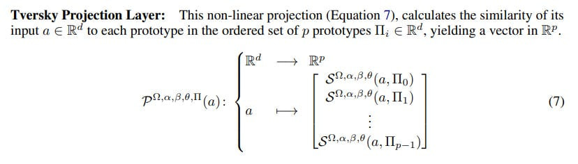
Tversky Projection Layer, analogous to a fully connected layer. A nonlinear projection of vector a∈Rd, computing the similarity of input a to each of p prototypes, each of which is Rd, so the output is vector Rp. Essentially, it projects the input vector onto a set of learned "prototypical" vectors Π. However, instead of simple scalar product, it uses a more complex and expressive nonlinear Tversky similarity function in the Tversky Similarity Layer.

In total, the learnable parameters in Tversky neural networks include:
prototype vectors, Π
feature vectors, Ω
weights α, β, θ
Π and Ω can be shared between different layers.
This new layer is inherently more powerful. The authors constructively show that a single Tversky projection layer can model the nonlinear XOR function, which is impossible for a single linear layer, demonstrating its increased expressive capacity.
However, there's a nuance here. The XOR example, where the input is a vector of two numbers between which XOR is performed, uses 11 learnable parameters. Well okay, one classical neuron can't do XOR, but a simple network with one hidden layer with two neurons and one output neuron already can, and it has only 6 learnable weights — two for each neuron, bias doesn't seem necessary. Even with bias, that's still 9 weights, less than 11. So it's a questionable advantage; I too can embed all this into one neuron of a new type and say it's more powerful.
And the learnable prototype and feature vectors in Tversky networks still need to be learned; not every initialization succeeded in the experiments. And the hyperparameters (number of vectors) need to be chosen somehow.
Replacing standard linear layers with Tversky projection layers leads to notable improvements in various domains:
Image Recognition: When adapting frozen ResNet-50 for classification tasks, using a Tversky projection layer instead of linear at the output (=Tversky-ResNet-50) led to accuracy improvements from 36.0% to 44.9% (NABirds) and from 57.4% to 62.3% (MNIST). On unfrozen networks, it's not as noticeable; when training from scratch, it's slightly more noticeable.
Language Modeling: When training GPT-2 small from scratch on the Penn Treebank dataset with shared (tied) prototypes, replacing linear layers with Tversky layers (=TverskyGPT-2) simultaneously reduced perplexity by 7.5% and reduced parameter count by 34.8%.
Prototype and feature vectors were initialized randomly everywhere. Product and ignorematch were used as reductions in intersections and differences.
Another useful property of the model is interpretability. Most modern XAI methods, such as LIME or Grad-CAM, are post-hoc, meaning they try to explain model decision-making from the outside, after it has been trained as a black box. Unlike them, the Tversky framework is interpretable by design. Its fundamental operations are based on psychologically intuitive concepts of common and distinctive features, providing a built-in, transparent language for explaining model reasoning.
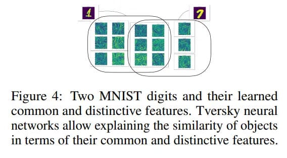
The authors present a new visualization technique in the input data space that allows visualizing learned prototypes and features directly in the input space. Using MNIST as an example, they show that the Tversky layer learns prototypes and features that correspond to recognizable, human-interpretable strokes and curves of handwritten digits. In contrast, the baseline linear layer learns opaque, uninterpretable textural patterns. This enables principled explanation of model decisions in terms of common and distinctive features.
The authors even discovered that trained models consistently learn parameters where α > β. This means that distinctive features of the input ("son") are given greater weight than distinctive features of the prototype ("father"). This is direct confirmation of Tversky's original salience hypothesis and shows that the model not only works well but also learns in a psychologically consistent manner.
Cool work overall. It begs for extension to transformers and attention mechanisms. In the paper, they only applied it to projection blocks.