Today we are announcing vector search in Onehouse Lakegres, with a native index stored inside existing and new open tables. You can search embeddings through a Postgres endpoint on the same tables you already have in your data lake. The index and data are managed in open formats in your own bucket.
Vector search stopped at the application database
A few years ago, adding vector search required a separate database. Postgres now has pgvector, OpenSearch has k-NN, and MySQL, Oracle, MongoDB and SQL Server have their own implementations. Databricks also offers vector search in Lakebase Search. Similarity search has become a standard index type for application data.
Most of the data an agent needs to query is in the lakehouse. Support transcripts, logs, documents, product catalogs and years of event history are stored in open tables on object storage. These datasets are 100 to 1,000 times larger than a typical Postgres instance. To search them with any of those databases, you have to copy the data into the database first. Copying lake-scale datasets into a relational database just to search their vectors is an absurd requirement. You end up paying to store the data twice and operating a pipeline to keep the copies in sync.
Yesterday, we announced unstructured data processing on Onehouse, which parses documents, images and video and stores their embeddings in open tables. Lakegres can now index and search those vectors, so agents can query that unstructured content alongside the business records already in the lakehouse.
How the market searches lake data today
Lakehouse and warehouse vendors have also added vector search. Each vendor below stores the index outside the open table, in a service or format that requires its own engine to read.
These vendors advocate open table formats while keeping their search indexes in closed formats. If you move to another engine, you have to rebuild every index in that vendor’s format, even though the underlying tables are open.
Why database techniques stop at lake scale
Most production vector search today runs on OpenSearch or Postgres. Both offer HNSW (OpenSearch implementation, pgvector implementation), a graph index that performs well when the entire graph fits in memory. AWS’s own sizing formula for OpenSearch is 1.1 × (4 × dimensions + 8 × m) bytes of RAM per vector. Our benchmark table has 247 million vectors at 1,024 dimensions. With m set to 16, that comes to about 1.15 TB of memory for one table, and about 46 TB at 10 billion vectors.
A pgvector HNSW index in Postgres also has to stay in shared buffers or the page cache to be fast, and latency degrades sharply once the working set exceeds RAM. Graph traversal is also a poor match for object storage, because each hop is a small random read. These designs work well for application databases with tens of millions of vectors. A data lake can be several orders of magnitude larger.
LinkedIn reported an exabyte across its Hadoop clusters in 2021. Uber’s lake holds 350 petabytes and ingests 6 trillion rows a day. Pinterest runs a 500-petabyte lake on Iceberg, and Netflix describes its Iceberg warehouse as exabyte scale. Embedding even a small fraction of these datasets produces billions of vectors. Keeping that many vectors in RAM is too expensive for most teams.
Training-data curation also needs large-scale similarity search. Post-training workflows can use it to select relevant examples and remove near-duplicates across large pools of candidate data. Repeated searches make cost per search matter as much as latency.
VAST, which supplies storage for AI training, uses a clustered vector index on flash in its distributed Element Store. Its launch material describes memory-resident indexes as prohibitively expensive at tens or hundreds of billions of vectors. turbopuffer also uses storage-based clustering. Lakegres applies this approach to existing Hudi and Iceberg tables through an open index.
What we built
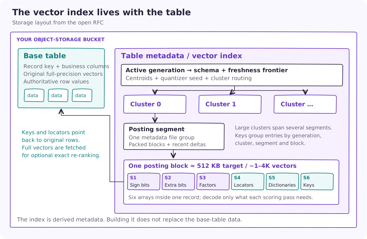
Lakegres stores the vector index in the table’s metadata, in the same bucket as the data files. Commits that insert, update or delete rows also update the index. This keeps the index consistent with the table without a separate sync job or a second copy of the vectors. To our knowledge, this is the only available open vector search index for existing Hudi and Iceberg tables that is maintained with table writes and leaves the data files unchanged.
Iceberg support builds on the Hudi-backed indexing work in Apache XTable (Incubating). We developed the design in the open with engineers from Uber and Walmart to support their planet-scale tables. The open RFC documents the storage layout, query path and consistency model.
The design is settled and ships in Lakegres today; the Hudi implementation is being upstreamed and XTable is in release-candidate testing ahead of OSS releases that other engines can integrate.
Lakegres accepts queries over the Postgres wire protocol, so any Postgres client or agent framework can run a similarity search in SQL. The same endpoint already serves analytical scans, indexed point lookups and text search on those tables.
How it works
Add or drop the index without rewriting the table
The vector index is derived metadata. You can build it on an existing Hudi or Iceberg table with a vector column without rewriting the underlying data files. You can experiment with an index, rebuild it with different settings, or drop it when you no longer need it. Existing analytical queries continue to work. Trying vector search costs you an index build and its storage.
You do not have to move from Parquet to another file format like Lance or Vortex just to get vector search. Lakegres also already queries Lance and Vortex files while keeping the open table format the same. You can choose a file format for its storage and read characteristics independently of adding a vector index.
The base table stores the full vectors alongside the other columns. The index stores the smaller structures needed to find candidate rows: cluster centroids, quantizer state and packed index entries. These structures are stored in the table’s metadata and grouped into an index generation. Each query resolves a table snapshot and an active generation before reading the data, so it uses a compatible set of index structures throughout.
Clusters divide the search space into bounded reads
At build time, k-means groups vectors around representative points called centroids. Each vector is assigned to a cluster and encoded relative to its centroid using RaBitQ quantization. The encoding uses a fixed random rotation and compact codes at 1 to 8 bits per dimension, with 4 bits as the default. The stored codes support L2, cosine and dot-product distance calculations.
Clusters are divided into posting segments, with each segment stored in one metadata file group. Within a segment, roughly 1,000 to 4,000 vector entries are packed into a posting block, targeting about 512 KB. A posting contains the compressed scoring information, record key and a locator for the underlying row. Grouping them into blocks avoids creating billions of individual metadata records and lets the query read a cluster’s entries as contiguous key ranges.

Each block contains separate arrays for sign bits, extra precision bits, correction factors, row locators, dictionaries and record keys. The first scoring pass decodes the sign bits and factors. Later passes decode extra bits and row identities only for surviving candidates. The reader fetches the block as one record, then selectively decodes its arrays to reduce scoring work.
A query narrows the candidates before it fetches full vectors
Lakegres first compares the query vector with the centroids and probes the nearest clusters. The nprobes setting controls how many clusters it opens. Probing more clusters generally improves recall at the cost of more work. Within those clusters, a first pass uses one-bit estimates and error bounds to discard candidates that cannot beat the current shortlist. A second pass uses the remaining bits to refine the surviving candidates.

Before returning results, the reader validates candidate keys against the record index at the query’s snapshot. Deleted candidates are removed and moved records are resolved to their current location. Approximate mode ranks the candidates with their compact codes. Optional exact re-ranking reads the shortlisted vectors from the base table and computes their full distances. Exact re-ranking improves the ordering within the candidate set. The search still examines only the selected clusters.
The index stays up to date as the table changes
Each write adds small updates to the index. When a vector changes, the writer marks its old index entry as deleted and adds a new entry. When a row moves, the writer updates its location in the index. Queries read the packed blocks and these updates together. They use the latest entry for each record. Compaction periodically merges the updates into the blocks.
Before searching, the reader checks the table’s commit history. It verifies that the index includes the writes required by the query’s snapshot. A stale or incompatible index cannot serve the query. Depending on the configuration, the query either returns an error or scans the table for exact results.
You can rebuild the index while queries continue to run. The concurrency protocol coordinates table writes, index catch-up and snapshot reads so writers can keep committing while readers continue using a consistent index. The rebuild creates a new index version alongside the current one. It also picks up table writes made during the rebuild. Once the new version is ready, a single metadata commit makes it available to queries. Queries use the current version until the new version is online atomically. They never read a partially built index.
Benchmarks
We used Cohere’s public multilingual Wikipedia embedding dataset. Our table contains 247,154,006 passages, approximately 247M vectors, with 1,024-dimensional embeddings generated by Cohere Embed v3. The table occupies about 1 TB on S3.
We designed Lakegres vector search for tables that grow to billions of vectors. We therefore compare against Databricks AI Search’s storage-optimized tier, its offering for large datasets. Its standard tier has a documented capacity of roughly 320M vectors at 768 dimensions, equivalent to about 240M at the 1,024 dimensions used here.
We ran the same workload on Lakegres and Databricks AI Search, the most directly comparable service for lake data. Each system ran the same 200 queries for the 10 nearest neighbors, one at a time. Recall was scored against exact brute-force results.

For warm queries, Lakegres returned results in 63.5 ms at p50, 67.9 ms at p90 and 75.3 ms at p99. Databricks AI Search took 655 ms, 876 ms and 1,209 ms, respectively. Cold p50 latency was 536.2 ms for Lakegres and 8,242 ms for AI Search. Recall@10 was 0.95 for Lakegres and 0.952 for AI Search.
Warm queries benefit from partially cached index data. Queries read the posting blocks for selected clusters, fetching blocks from storage when they are not cached. The full vector dataset stays in the table and does not need to fit in memory.
Lakegres uses a configurable compute cluster. Databricks AI Search serves a separate index through a serverless endpoint, with capacity automatically sized for the indexed data.
Lakegres ran on five m8gd.4xlarge executor nodes and one r8gd.4xlarge driver. AI Search ran on six storage-optimized units with one replica, and its hardware is not visible to customers. We used Databricks’ server-side latency measurements for AI Search and client-side psql timings for Lakegres. The two measurements therefore cover different parts of query execution. In a preliminary standard-tier test on a smaller, 10-million-vector table, the index build ran at about 70,000 rows a minute before we stopped it; we did not measure query latency on that tier.
Lakegres is about 10 times faster at the warm median and 15 times faster cold. The AWS instances cost about $5.79/hour at US East on-demand rates, excluding Onehouse fees; the six AI Search units cost $7.68/hour. These figures show the modest infrastructure budget behind the Lakegres result. They are not a total-cost comparison.
We expect similar query latency on multi-billion-vector tables as we scale out Lakegres. This run used just five Spark executors plus a driver. As a table grows, we can increase the number of index clusters and distribute posting-block reads and scoring across more workers. Each query still searches selected clusters, and workers can fetch the required blocks from storage without loading the entire index into memory. This gives us control over the work per worker as the dataset grows. We will publish results on much larger vector datasets in follow-up blogs.
In a separate index-build benchmark, building the index took 18 minutes on Lakegres and about 3 hours 10 minutes on AI Search. Lakegres builds the index on the lakehouse’s elastic compute, so you can increase the cluster size to build it faster. AI Search provides no control over build cluster size and reports progress only as a percentage.
Dedicated vector-search systems and storage platforms also publish retrieval latency figures. The table below lists their reported results on different datasets and hardware, with different dimensions, latency metrics and query concurrency.
Get started
Create the index with a CREATE INDEX statement. These are the options we used for the benchmark table.
CREATE INDEX embedding_idx ON wiki_passages
USING VECTOR (embedding)
OPTIONS (
  `vector.metric` = 'l2',
  `vector.num_clusters` = '65536',
  `vector.rabitq.bits` = '4'
);
To search, call the table function from any Postgres client. It returns the nearest rows and their distances. The nprobes option controls how many clusters the query opens, which is the main tradeoff between latency and recall.
SELECT id, _distance
FROM vector_search(
  'wiki_passages', 'embedding',
  ARRAY[0.12, -0.03, 0.44],   -- the query embedding, shortened here
  10, 'l2', 'ivf_rabitq_mdt',
  'vector.query.nprobes=128'
);
Where we’re headed
Most of the remaining latency difference from the fastest dedicated systems comes from work outside the index. Roughly 20 to 25 ms of each query is spent in Spark, in planning and task scheduling, before any index block is read. We saw the same fixed overhead, in the tens of milliseconds, when testing Trino and other lake engines. These engines were built to plan large scans. We have designed a way to remove this overhead from index lookups and plan to implement it next.
The first release supports filtering through partition pruning. It does not support arbitrary predicates combined with nearest-neighbor search. If the cluster layout drifts from the data, you can rebuild the index while queries continue, then activate the new generation atomically.
Conclusion
Agents need four kinds of queries from a data platform: analytical scans, indexed point lookups, text search and vector search. Lakegres now serves all four from one copy of your open tables, through one Postgres endpoint, as the platform guide describes.
Try Lakegres vector search on your own tables with a free test drive. Our engineers are also in the Onehouse community Slack if you want to talk through your use case.
Acknowledgments
The index’s storage layout, consistency guarantees and query behavior were developed and reviewed in public through the open RFC and implementation PRs. The community can inspect, implement and improve the indexes as well as the table format they depend on.
We thank Ethan Guo, Vinoth Chandar and Revanth, a Walmart engineer and Apache Hudi contributor, for their contributions to the vector index design and implementation.
We also thank @rahil-c, @nsivabalan, @sushrut-raina, @voonhous, @danny0405, @TheR1sing3un, @suryaprasanna, @bvaradar, @shangxinli and @cshuo for their reviews of this deep, critical feature.