I was recently trying to simplify convex hulls. A common approach is to find all the face planes of the hull, merge or drop some of them, and then rebuild the hull from the planes that are left. There are two common ways to do the rebuild. The first is to make each plane a giant quad and clip it by every other plane, repeating this for each plane. The second is to take the convex hull of the face normals. Each face plane \(\boldsymbol{n \cdot x = d}\) becomes the point \(\boldsymbol{n/d}\), so this is the convex hull of the dual polytope, and its faces give the vertices of the simplified hull. I had trouble understanding the dual polytope, so this is a short explanation of it in terms of the level sets of the support function.
Let \(\boldsymbol{P}\) be a convex polytope with vertices \(\boldsymbol{v_{1}, v_{2}, \dots v_{k}}\) and the origin inside it. Its support function is
\[h(y) = \max_{x \in P} (x \cdot y) = \max_{i} (v_i \cdot y)\]
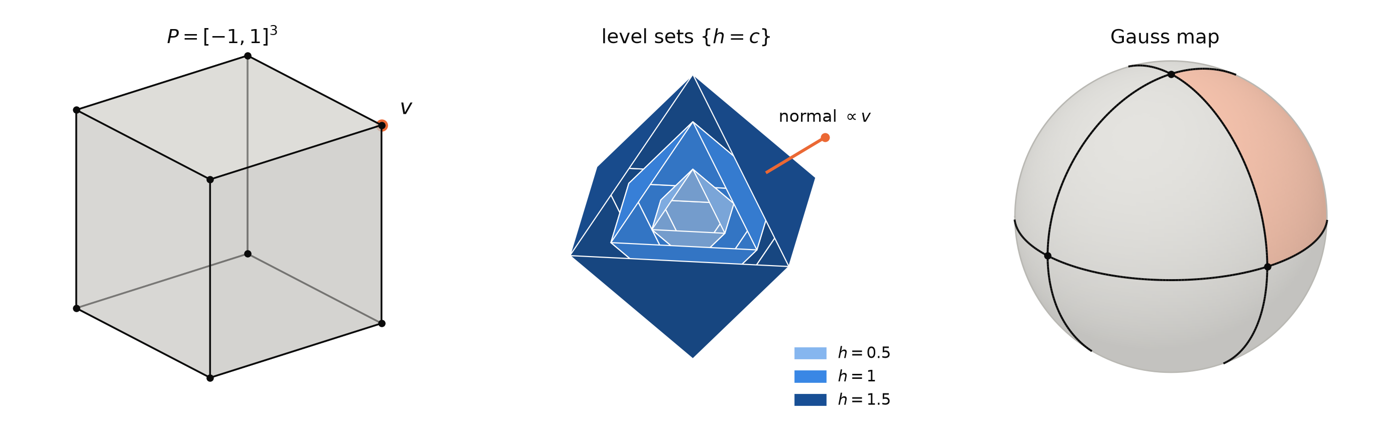
The support function is piecewise linear. Its linear regions are wedges, one per vertex, where wedge \(\boldsymbol{i}\) is the set of directions whose support vertex is \(\boldsymbol{v_{i}}\). On the sphere these wedges are the regions of the Gauss map. Let’s look at the level sets of \(\boldsymbol{h}\).

Since \(\boldsymbol{h}\) is linear inside each wedge, a level set of \(\boldsymbol{h}\) is flat inside each wedge and can only bend on the seams between wedges. From that, these properties should be clear.
The wireframe of a level set projects onto the Gauss map.
Its faces sit over the regions of the Gauss map, one per vertex of \(\boldsymbol{P}\).
Its vertices sit over the points where the arcs meet, one per face of \(\boldsymbol{P}\).
The polar dual of \(\boldsymbol{P}\) is
\[P^{\circ} = \{y : x \cdot y \leq 1,\ \forall x \in P\}\]
Theorem. For \(\boldsymbol{c > 0}\) the level set \(\boldsymbol{\{h \leq c\}}\) is \(\boldsymbol{cP^{\circ}}\), and
\(\boldsymbol{P^{\circ}}\) is a convex polytope.
The faces of \(\boldsymbol{P^{\circ}}\) are the vertices of \(\boldsymbol{P}\). Face \(\boldsymbol{i}\) lies in the plane \(\boldsymbol{v_{i} \cdot y = 1}\), so its normal is \(\boldsymbol{v_{i}}\).
The vertices of \(\boldsymbol{P^{\circ}}\) are the faces of \(\boldsymbol{P}\). A face of \(\boldsymbol{P}\) with plane \(\boldsymbol{n \cdot x = d}\) becomes the vertex \(\boldsymbol{n/d}\), and projecting the edges of \(\boldsymbol{P^{\circ}}\) onto the sphere gives the Gauss map.
Proof. From the definition of \(\boldsymbol{h}\),
\[h(y) \leq 1 \iff x \cdot y \leq 1 \ \text{ for all } x \in P\]
so \(\boldsymbol{\{h \leq 1\} = P^{\circ}}\). Since \(\boldsymbol{h(ty) = t\,h(y)}\) for \(\boldsymbol{t > 0}\), the other level sets are scaled copies,
\[\{h \leq c\} = cP^{\circ}\]
Since \(\boldsymbol{h}\) is a max of linear functions,
\[P^{\circ} = \bigcap_{i} \{y : v_{i} \cdot y \leq 1\}\]
is an intersection of finitely many half spaces. It is bounded because the origin is inside \(\boldsymbol{P}\), so
\[h(y) \geq m \lVert y \rVert, \qquad m = \min_{\lVert y \rVert = 1} h(y) > 0\]
On wedge \(\boldsymbol{i}\),
\[h(y) = v_{i} \cdot y\]
so inside that wedge the boundary of \(\boldsymbol{P^{\circ}}\) is the plane \(\boldsymbol{v_{i} \cdot y = 1}\). Different vertices give different planes, so neighbouring faces meet at an angle along the seams.
By homogeneity every ray from the origin crosses the boundary of \(\boldsymbol{P^{\circ}}\) exactly once, at \(\boldsymbol{y/h(y)}\). So projecting onto the sphere sends each face of \(\boldsymbol{P^{\circ}}\) to its wedge and each edge to a seam, which is the Gauss map. The vertices of \(\boldsymbol{P^{\circ}}\) lie where three or more wedges meet, which is along the face normals \(\boldsymbol{n}\) of \(\boldsymbol{P}\). Along that ray
\[h(tn) = t\,d = 1 \implies t = \frac{1}{d}\]
so the vertex is \(\boldsymbol{n/d}\). \(\blacksquare\)
Merging or dropping face normals edits the vertices of \(\boldsymbol{P^{\circ}}\), and taking their convex hull rebuilds \(\boldsymbol{P^{\circ}}\). By part 2 of the theorem, each face \(\boldsymbol{w \cdot y = 1}\) of the new hull gives the vertex \(\boldsymbol{w}\) of the simplified polytope.