July 19, 2026 at 9:07 PM by Dr. Drang
Yesterday I watched the most recent Numberphile video, in which Ben Sparks explains a few finite series and the equations that simplify the calculation of their sums. He derives the formulas graphically, and it’s all very cleverly done, especially the one for the sum of cubes.
The idea is to get a simple polynomial expression in n for
As I said, Ben’s graphical method is really clever and easy to understand, and it leads to this expression:
I wanted to see if I could get that same result using a nongraphical and less clever method. The method that came to mind was to generate a handful of values, put them in a table, and start taking differences.
Here are some values of n, N, and the first four differences:
| n | N | Δ | Δ² | Δ³ | Δ⁴ |
|---|---|---|---|---|---|
| 1 | 1 | 8 | 19 | 18 | 6 |
| 2 | 9 | 27 | 37 | 24 | 6 |
| 3 | 36 | 64 | 61 | 30 | |
| 4 | 100 | 125 | 91 | ||
| 5 | 225 | 216 | |||
| 6 | 441 |
The differences are calculated by looking in the preceding column and subtracting the value in the same row from the value in the following row. This sort of thing is fairly easy to do by hand but is really easy to do in a spreadsheet. Here’s a screenshot of the table in Numbers, where I’m displaying the formula for the first difference, Δ:
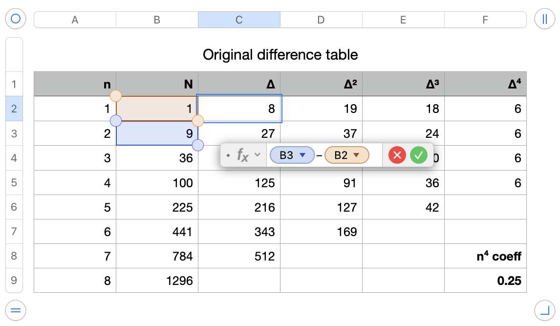
That formula can be filled into all the difference cells, which is why it’s so easy. (I included only the first six rows in the table above because I figured you’d trust me that all the values in the fourth difference column, Δ⁴, are the same.)
The constant values in the fourth difference column mean N is a fourth-degree polynomial in n:
Because the constant fourth difference is 6, we know that
This comes from the fact that differences are analogous to derivatives, and
Once we know the degree of the polynomial and have , we can figure out the other coefficients by solving a set of four simultaneous equations for four different values of n and N. For example:
We could use any four of the six Ns we’ve calculated, but the first four are convenient. Let’s solve them in Python using NumPy and the solve function from the linalg submodule. We can do this interactively:
python:
from numpy import np

m = np.array([[1, 1, 1, 1], [1, 2, 4, 8], [1, 3, 9, 27], [1, 4, 16, 64]])
b = np.array([1 - 1**4/4, 9 - 2**4/4, 36 - 3**4/4, 100 - 4**4/4])
np.linalg.solve(m, b)
The last line returns
python:
array([ 1.77635684e-15, -3.99680289e-15,  2.50000000e-01,  5.00000000e-01])
Those first two elements of the solution array are at the lower limit of what a floating point number can be. So we can say
Therefore,
or, after collecting terms,
which is the formula Ben got in the video.
Doing basically the same thing in Mathematica is
m = {{1, 1, 1, 1}, {1, 2, 4, 8}, {1, 3, 9, 27}, {1, 4, 16, 64}};
b = {1 - 1^4/4, 9 - 2^4/4, 36 - 3^4/4, 100 - 4^4/4};
LinearSolve[m, b]
which returns
{0, 0, 1/4, 1/2}
This is the same as the Python answer but with no need to think about floating point precision.
A third way to solve the simultaneous equations is to do it in a spreadsheet. Here’s how that looks in Numbers:
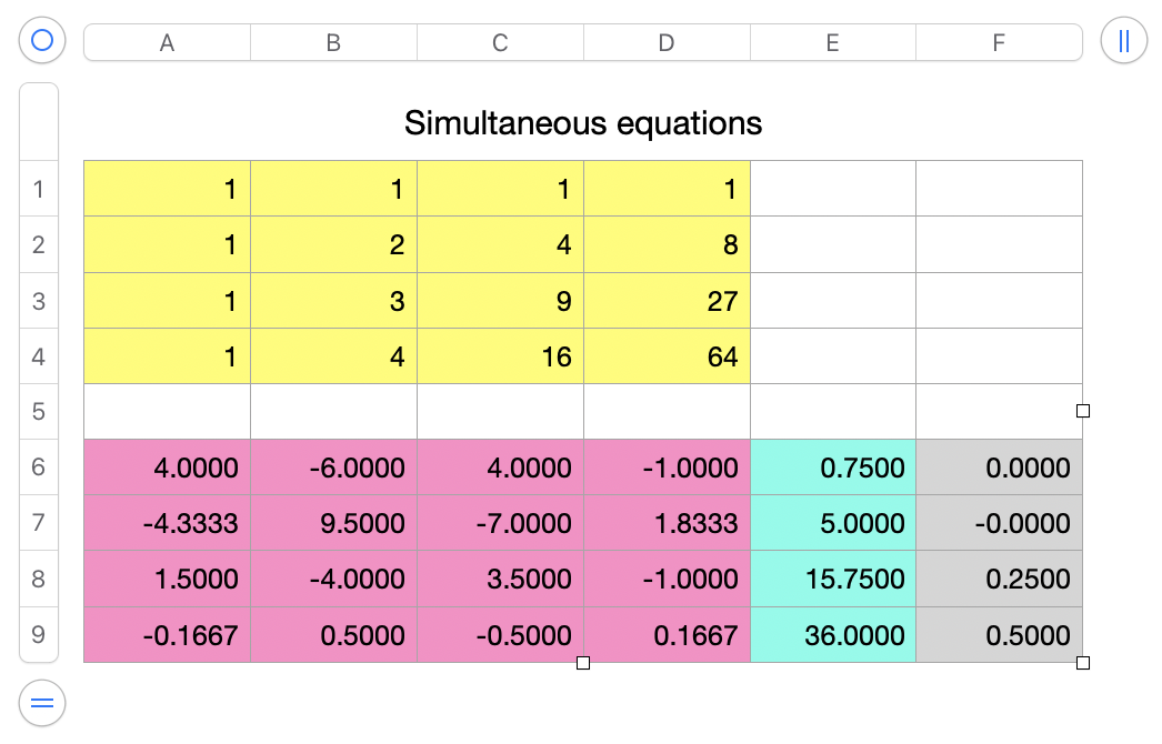
where
- the block of yellow cells is the matrix
min the Python and Mathematica solutions; - the block of magenta cells is the inverse of
m; - the block of cyan cells is the vector
bin the Python and Mathematica solutions; and - the block of gray cells is the solution for through , determined by multiplying the magenta matrix by the cyan vector.
The spreadsheet uses a combination of MINVERSE and MMULT, functions that are also in Excel and Google Sheets. As with the Python solution, there are floating point artifacts here. They’re mostly hidden by my choice to show only four decimal places, but that -0.0000 for is a clue that these are not exact answers.
You might well ask why I’d bother using Python or Mathematica to solve the simultaneous equations if I already had a spreadsheet open to make the difference table. The answer is that I generally prefer working in an environment where my formulas and expressions are always visible. It makes things easier to debug, and I’m always debugging.
There are other ways to determine the coefficients. My favorite is a step-by-step procedure that simplifies the problem one polynomial degree at a time.
Given that we know from the difference table above, we can make a new table for
and its differences. By subtracting the fourth-degree term from N, we expect P to be a third-degree polynomial. Here are the first five rows of the difference table for P:
| n | P | Δ | Δ² | Δ³ |
|---|---|---|---|---|
| 1 | 0.75 | 4.25 | 6.50 | 3.00 |
| 2 | 5.00 | 10.75 | 9.50 | 3.00 |
| 3 | 15.75 | 20.25 | 12.50 | |
| 4 | 36.00 | 32.75 | ||
| 5 | 68.75 |
As expected, they become constant at the third difference. Using the same technique we used to get , we can say
Moving on, we make a table for
and its differences. Here are the first four rows of that table:
| n | Q | Δ | Δ² |
|---|---|---|---|
| 1 | 0.25 | 0.75 | 0.50 |
| 2 | 1.00 | 1.25 | 0.50 |
| 3 | 2.25 | 1.75 | |
| 4 | 4.00 |
These become constant at the second difference, and we can say
Finally, we make a table for
which is this:
| n | R |
|---|---|
| 1 | 0.00 |
| 2 | 0.00 |
| 3 | 0.00 |
| 4 | 0.00 |
Since all the R values are zero, the rest of the coefficients, and , must be zero, and we’re done.
If it’s not obvious why , consider this:
The only way for R to be zero for all values of n is if .
Building these tables is fairly easy, but it’s not as fast as building and solving the simultaneous equations. Still, there’s some satisfaction in marching to the answer this way. It’s basically a recursive solution, where we’re simplifying the problem with each step.
Using difference tables to work out the formula for the sum of cubes isn’t as slick as the graphical method shown in the video, but it does have the advantage of not requiring any ingenuity. I’m not opposed to ingenuity, but sometimes you want to just set the problem up, turn the mathematical crank, and get the answer.