Fall Semester 2020
Morphometrics, Functional Morphology & Biomechanics
Key Points:
•Morphometrics is the quantitative study of form. There are many available morphometrics to study form and its change with ontogeny, evolution, taphonomy, etc.
•Principal Components Analysis (and its close cousing Principal Coordinates Analysis) are the real workhorse methods in morphometrics, summarizing multiple variables at once.
•Morphospaces are the expression of quantified shape into graphical form. There are both theoretical (mathematical) morphospaces, determined by a priori selection of the axis variables; and empirical morphospaces, derived directly from the morphometric analysis results.
•Our ability to reconstruct the function of extinct forms comes through multiple lines of evidence: analogies with the function in extant animals with similar forms; phylogenetic inferences such as the extant phylogenetic bracket method; biomechanics and other cases of modeling; trace fossil analyses; and correlations between phenomena.
•That said, not all form is functional. Some features at least start as "spandrels": the byproduct of the constructional development of the organism rather than actively-selected traits.
"If you want to inspire confidence, give plenty of statistics. It does not matter that they should be accurate, or even intelligible, as long as there is enough of them." -- La poétique de l'espace, Gaston Bachelard (1958)
MORPHOMETRICS: INTRODUCATION TO THE ANALYSIS OF SHAPE
We encourage everyone interested in this subject to examine the excellent "PalaeoMath" series of articles by Norm MacLeod. Furthermore, for those interested in exploring these techniques directly, please check out the following software packages:
Note that these notes are by no means comprehensive: you can take (literally) entirely courses on morphometrics, statistical analyses, and functional morphology.
We have seen the Raupian attempt to reduce morphological variation to a small number of parameters. In all but the simplest systems, such a method greatly oversimplifies morphology. Nevertheless, the need to describe morphology with quantitative rigor is fundamental to descriptive paleontology, and to the testing of hypotheses of functional morphology. In this lecture we consider morphology and function separately.
Morphometrics: The quantitative study of form, including both size and shape. Fundamental to the description of individual specimens and collections of specimens in order to: recognize the degree of distinctiveness of different morphs (which might be age stages, sexes, taxa, etc.); trace changes due to evolution, ontogeny, etc.; and to remove the disruptive effects of taphonomy by retrodeformation back to the original shape.
Traditional morphometrics: Measurements that have become standardized for the description of morphology through tradition, usually owing to their lack of ambiguity. Naturalists have been using calipers to obtain quantitative information about morphology for centuries. That information has been fed into multivariate statistical analyses for a full century. These begin to enable us to describe distributions of morphological variation.
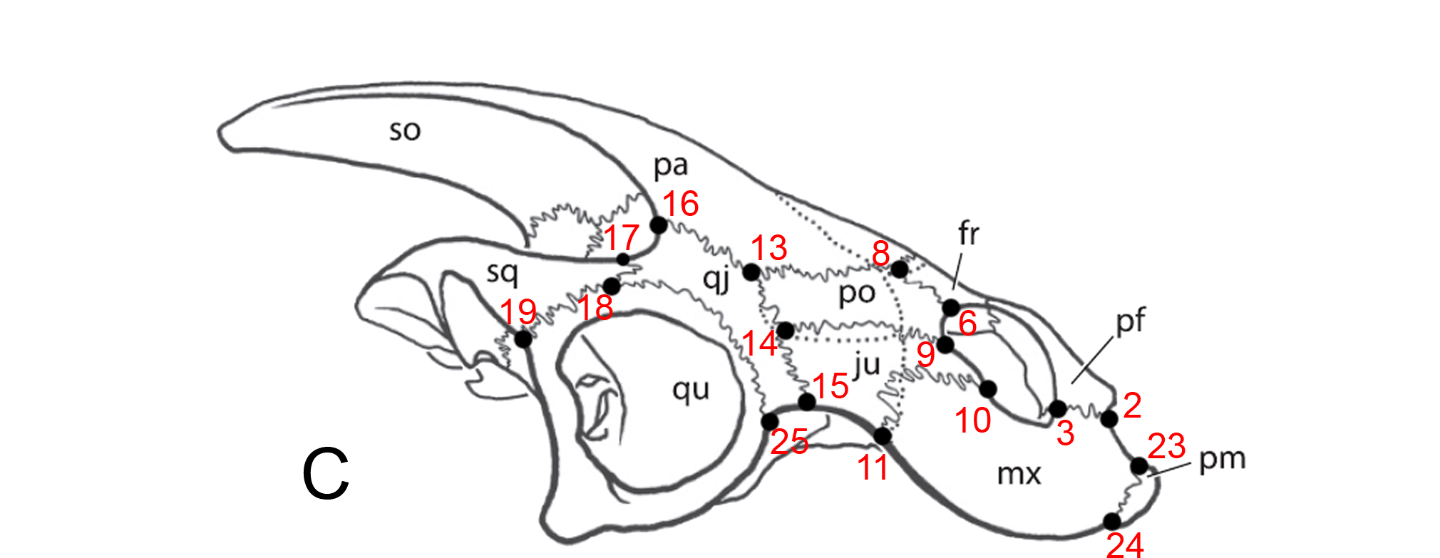
The key here is to develop and recognize landmarks: points on a body (often where bones or other body parts join together) which can be compared from one specimen to another.
But what do the data actually mean? In traditional morphometrics, data are measurements of the distances between points on a specimen. These points may be:
- Landmarks: Discrete points marked by homologous features (right - red) like:
- Foramina
- Intersections of sutures in bones
- Branching points of veins
- Other similar points
- Semilandmarks: Arbitrary points on the exterior margin describe shape but may be non-homologous (right - blue) like:
- points of maximum width
- the tips of snouts
- etc.
One of the most standard of all statistical analyses is:
Phylogenetic Considerations: Biologists are fond of performing statistical studies, looking for meaningful correlations between measurable aspects of different parts of animals' anatomies. For instance, one might look at the ratio of the length and depth of birds' beaks vs. the length of their tarsals to see if larger birds have proportionately deeper beaks. Measurements of this sort can be subjected to the full range of statistical analyses. A fundamental assumption of such studies is that all observations be made from independent members of the same underlying population.
However, when samples are being taken from groups of populations nested in a hierarchical phylogeny, this assumption is violated. The example at right shows of how misleading this can be. Imagine a simple phylogeny with two sister clades, one black, the other red. When we make a bivariate plot of data taken from them, there appears to be a strong statistical relationship. But in fact, when we compare values only within each clade, we see very low correlation.
Fortunately, Joe Felsenstein of the University of Washington provided a first attempt at a solution in a statistical technique for adjusting data to account for the phylogeny of the taxa sampled, called phylogenetically independent contrasts (PIC). This method is based on the concept that although the taxa may be non-independent, the differences between measured values in them are independent. Statistical correlation techniques are, therefore, applied to pairwise contrasts in measurements from sister taxa. By applying it, meaningful correlation studies can be performed. Without it, they would be meaningless or misleading. Applying this method absolutely requires a known phylogeny. If hypotheses of phylogeny change, the results of correlation studies based on them must be revised, too.
Work in subsequent decades have recognized Felsenstein's method is just one of multiple alternative solutions with different models of evolutionary change. Many additional alternative statistics have been developed, depending on the model of evolution assumed in a given situation.
PRINCIPAL COMPONENTS ANALYSIS (PCA)
What if you are interested in examining many variables in the same system? You can do a series of bivariate plots, doing each possible pair of variables as its own graph. As the number of variables increases, though, this becomes difficult to interpret. One could to a trivariate plot (XYZ plot), but these can be difficult to interpret (you need to move the figure around to get the sense of the distribution of data), and only gets you one more variable. Thankfully, there is a good way of boiling down multiple variables into a more simplified format.
- The first principal component represents the primary source of variation, the second, the secondary, etc. Indeed, you can recognize HOW MUCH of the variation is explained by each component.
- There can be as many principal components as there are variables.
- The principal components, being mutually perpendicular, are not correlated with one another.

PCA need not be done only on morphometrics. For instance, ecologists and paleoecologists often use abundance data of species (where localities are the object of study and the abundance of each species is the variable) to find similarities and dissimilarities between localities.
A related technique is Principle Coordinate Analysis, which doesn't require that every cell in your measurement matrix is occupied.
This may be trivial for a bivariate plot, but discriminant function analysis also works for multivariate analyses in many dimensions, where data cannot be as easily visualized.
Thompson was fond of expressing morphological variation in terms of "transformations" - by which the shape of one species could be transformed into that of another by the application of regular simple transformations, reflected as deformed grids. (E.g. puffer and mola, right.) Although clever and not lacking merit, these reflected a level of subjectivity. Indeed, the technique was pioneered by the Renaissance artist Albrecht Dürer. They pointed out the need for an algorithmic approach to the quantitative analysis of shape, however, which were finally developed in the 1980s and 1990s. Here is a synopsis of what has emerged.

Landmark-based analysis: Dismisses the measurements of traditional morphometrics and focuses on the distribution of the landmarks - homologous identifiable points in sets of comparable samples. Landmark positions are first recorded as cartesian coordinates, thus preserving information about shape.
Example: For illustration, we show three specimens with different shapes. In practice, a normal data set would contain more. Constraints:
- The data must reflect shape adequately.
- Comparable landmarks must be present on all specimens.
- The number of specimens required depends on the size of the difference you seek to study compared to the amount of variation in your group.
Step 1: Data acquisition. Can be through:
- Calipers, steel tape, etc. on the real specimen
- Digital measurements on images of the same
Step 2: Procrustes superimposition. A series of steps in which size, positional, and orientation data are removed, leaving only shape.
- Centroids calculated for all shapes
- Size and orientation normalized using least squares concept.
Step 3: Principal Component Analysis. With size and orientation information removed, landmarks can now be treated as variables in PCA. The results map non-correlated sources of variation in shape without respect to size. This can be explored graphically with reference to the original data (right) or through thin-plate spline grids.

Outline-based analysis: An alternate approach involves describing the outline of an object mathematically by the fitting of coefficients of mathematical functions to a regular array of preset semilandmarks around the outline. In this case, there is no expectation that the points represent homologous features.
-
Eigenshape analysis: A common method of mathematical description is eigenshape analysis, in which a preset number of regularly spaced semilandmarks approximate the object's shape. For each semilandmark, the deviation of the angle of the line connecting it to the next from a circle centered on the centroid is recorded for each semilandmark, becoming a variable in a PCA, whose results can be expressed graphically.

For closed curves, Elliptical Fourier analysis: (Not pictured) In which the shape of the outline is approximated by the sum of the minimum number of ellipses needed to mimic its shape. This only works on outlines that are consistently convex.
Morphometrics in three dimensions: Most of the techniques discussed here can in principle be adapted for use with three-dimensional objects, although logistics become more complex.
Data acquisition: Depending on the size of the subject:
- Reflex microscopes
- Microscribe robotic arms
- Laser scanners
- CT scanners
MORPHOSPACE
A morphospace is an n-dimensional representation of possible form, shape, or structure of organisms. Each axis represents some variable describing the organism (either the raw variable, or a transformed component/coordinate). The point in morphospace represents an individual or an averaged representation of a taxon.
Raup's 3D morphospace for conical shells is a classic example of a morphospace in paleontology and zoology:

From Raup, D.M. 1966. Geometric analysis of shell coiling: general problems. Journal of Paleontology 40: 1178-1190.
In this space, the axes represent the translation of the aperture (x), the expansion of the aperture (y), and the distance of the generating curve from the axis (z). The fields represent the distribution of known shells (of mollusks and brachiopods) within this morphospace.
Raup's morphospace is an example of a theoretical (or mathematical) morphospace. The axes are pre-determined paramaters, allowing for all possible ranges of morphological variability to be expressed by systematically varying the values. It may be that some of the space is not occupied at all. One advantage of this sort of morphospace is that it is set up "in advance" of any analysis, as it were. The axes are not contingent on the measurements you take, and you can free add to the plots with new specimens as you discover them. A disadvantage is that it requires you to develop the parameters in advance: in reality, you might not really know which measured variables really are the most significant (i.e., explain the most data range) in your sample.
In order to address this problem, many choose to use empirical morphospaces. In these the axes are derived from statistical analyses of the actual specimens (typically a PCA or Principal Coordinate analysis). Thus the axes of the morphospace are the most significant ones within the population of data you sampled, and the morphospace is likely to be more greatly occupied. A disadvantage, however, is that the axes are analysis-dependent; you can't just pop new measurements onto your current plot. Instead, you would need to rerun the entire analysis and replot the whole set of data.
Revisiting the issues of theoretical morphospace: why might it be that some parts of it are not occupied by known taxa? Several ideas have been proposed (and, as usual, are not mutually exclusive):
- Mechanical limitations: it might be that certain combinations of variables simply do not work (i.e., are too fragile; cannot actually be generated by the biological system; etc.)
- Nature simply hasn't had time to fill in those spots
- In order to get into those regions, evolution would have to move "downslope" on an adaptive landscape
- Also called fitness landscapes, these are graphical metaphors proposed by leading New Synthesis proponent Sewell Wright.
- Under this concept, there is a "landscape" of peaks (of high fitness) and valleys (low fitness). Populations can only evolve towards adaptive peaks: to do otherwise would mean that the population is moving towards reduced fitness.
- Selection (under ordinary circumstances) can only move towards local optima.
- But large mutational jumps might get you "over" a peak onto the slopes of an even steeper (more highly adaptive) one
- And the landscape itself changes as the environmental conditions change (i.e., what is favored by selection)
Note that morphospaces might be used to explore the ecology in which an organism occupies as much as its shape.
To Syllabus.
Last modified: 7 December 2020