Let us begin with a simple example: a one-dimensional radar that measures range and velocity by transmitting a pulse toward an aircraft and receiving the reflected echo. The time delay between pulse transmission and echo reception provides information about the aircraft range \(r\), and the frequency shift of the reflected echo provides information about the aircraft velocity \(v\) (Doppler effect).

In this example, the system state is described by both the aircraft range \(r\) and velocity \(v\). We define the system state by the vector \(\boldsymbol{x}\), which includes both quantities:

\[ \boldsymbol{x}=\left[\begin{matrix}r\\v\\\end{matrix}\right] \]

We denote vectors by lowercase bold letters and matrices by uppercase bold letters.

Because the system state includes more than one variable, we use linear algebra tools, such as vectors and matrices, to describe the mathematics of the Kalman Filter. If you are not comfortable with linear algebra, please review the One-Dimensional Kalman Filter section in the online tutorial or in the book. It presents the Kalman Filter equations and their derivation using high-school-level mathematics, along with four fully solved examples.

Iteration 0

Filter initialization

In this example, we will use the first measurement to initialize the Kalman Filter (for more information on initialization techniques and their impact on the Kalman Filter performance, refer to Chapter 21 of the book). At time \(t_0\), the radar measures a range of \(10,000m\) and a velocity of \(200m/s\). The measurements are denoted by the letter \(\boldsymbol{z}\).
We stack the measurements into the measurement vector \(\boldsymbol{z}\):

\[ \boldsymbol{z}_0=\left[\begin{matrix}10{,}000\\200\\\end{matrix}\right] \]

The subscript \(0\) indicates time \(t_0\).

The measurement does not reflect the exact system state. Measurements are corrupted by random noise; therefore, each measurement is a random variable.

Can we trust this measurement? How certain is it? Each measurement is accompanied by a squared measurement uncertainty value (sometimes called the measurement error). This squared uncertainty is the measurement's variance. You can read more about variance in the Essential Background I section. For a more detailed discussion of measurement uncertainty, see the Kalman Filter in One Dimension section.

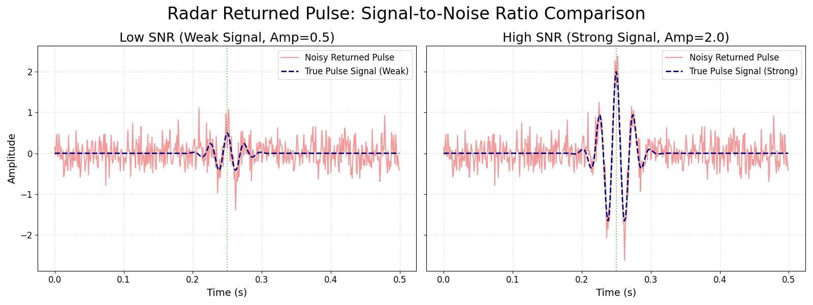
In radar systems, measurement uncertainty is largely determined by the ratio of received signal strength to noise. The higher the signal-to-noise ratio, the lower the measurement variance, and the greater our confidence in the measurement.

The following figure compares low-signal and high-signal cases in the presence of noise.

Let us assume that the standard deviation of the range measurement is \( 4m \) and the standard deviation of the velocity measurement is \( 0.5m/s \). Since variance is the square of the standard deviation, the squared measurement uncertainty (denoted by \( \boldsymbol{R} \)) is:

\[ \boldsymbol{R}_0=\left[\begin{matrix}16&0\\0&0.25\\\end{matrix}\right] \]

\( \boldsymbol{R} \) is a covariance matrix. The main diagonal elements contain the variances, and the off-diagonal elements are the covariances between measurements.

\[ \boldsymbol{R}=\left[\begin{matrix}\sigma_r^2&\sigma_{rv}^2\\[0.5em]\sigma_{vr}^2&\sigma_v^2\\\end{matrix}\right] \]

In this example, we assume that errors in the range and velocity measurements are not related to each other, so the off-diagonal elements of the measurement covariance matrix are set to zero.

For a refresher on variance and standard deviation, see the Essential Background I section of the online tutorial.
For a refresher on covariance matrices, see the Essential Background II section.

During initialization, the only information we have is a single measurement. In this example, the measurement and the system state are described by the same quantities (\(r\) and \(v\)). Therefore, we can use the measurement as the initial estimate of the system state. This can be done only during the initialization step:

\[ \boldsymbol{\hat{x}}_{0,0}=\boldsymbol{z}_0=\left[\begin{matrix}10{,}000\\200\\\end{matrix}\right] \]

Note: a caret (or hat) over a variable indicates an estimated value.

The subscript \(0,0\) has the following meaning:

• The first index refers to the time of the system, which in this example is \(t_0\).
• The second index refers to the time at which the estimate was made, which is also \(t_0\).

In other words, the estimate is for time \(t_0\), and it was also calculated at the time \(t_0\).

Prediction

We now predict the next state. Assume the target revisit time is 5 seconds \((\Delta t=5s)\), therefore \(t_1=5s\).

To estimate the future system state, we must describe how the system evolves over time. In this example, we assume a constant velocity dynamic model (the motion model):

\[ v_{1} = v_{0} = v \] \[ r_{1} = r_{0} + v_{0}\Delta t \]

(For examples of accelerating dynamic models, refer to Chapter 9 of the book.)

Let us describe the dynamic model in a matrix form:

\[ {\hat{\boldsymbol{x}}}_{1,0}=\boldsymbol{F}{\hat{\boldsymbol{x}}}_{0,0} \]

The subscript \(1,0\) has the following meaning:

• The first index refers to the system time, which is \(t_1\).
• The second index refers to the time at which the estimate was made, which is \(t_0\).

Thus, \( \hat{\boldsymbol{x}}_{1,0} \) is our estimate of the system state at time \(t_1\), computed using information available at time \(t_0\). In other words, it is a prediction of the future state.

The matrix \( \boldsymbol{F} \) is called the state transition matrix and describes how the system state evolves over time:

\[ {\hat{\boldsymbol{x}}}_{1,0}=\left[\begin{matrix}{\hat{r}}_{1,0}\\{\hat{v}}_{1,0}\\\end{matrix}\right]=\left[\begin{matrix}1&\Delta t\\0&1\\\end{matrix}\right]\left[\begin{matrix}{\hat{r}}_{0,0}\\{\hat{v}}_{0,0}\\\end{matrix}\right]=\left[\begin{matrix}1&5\\0&1\\\end{matrix}\right]\left[\begin{matrix}10,000\\200\\\end{matrix}\right]=\left[\begin{matrix}11,000\\200\\\end{matrix}\right] \]

Appendix C of the book describes a method for modeling the dynamics of any linear system.

The equation

\[ {\hat{\boldsymbol{x}}}_{n+1,n}=\boldsymbol{F}{\hat{\boldsymbol{x}}}_{n,n} \]

is the state extrapolation (prediction) equation. It tells us how to compute the next state from the current one. It takes our current state estimate and uses the system's motion model to predict the state at the next time step.

The full form of the state extrapolation equation is:

\[ {\hat{\boldsymbol{x}}}_{n+1,n}=\boldsymbol{F}{\hat{\boldsymbol{x}}}_{n,n} + \boldsymbol{G}\boldsymbol{u}_n \]

where:

• \(\boldsymbol{u}_{n}\) is an input variable
• \(\boldsymbol{G}\) is an input transition matrix

The input vector represents additional information provided to the Kalman Filter, such as readings from an onboard accelerometer.

In this simple example, we assume there is no input, so \(\boldsymbol{u}_n=0\).

For an example that includes an input term, see the State Extrapolation Equation page of the online tutorial or the fully solved Example 10 in the book.

Every measurement and every estimate in the Kalman Filter comes with uncertainty information. After predicting the next state, we should also ask: how precise is this prediction?

The squared uncertainty of the current state estimate is represented by the covariance matrix:

\[ \boldsymbol{P}_{0,0}=\left[\begin{matrix}16&0\\0&0.25\\\end{matrix}\right] \]

However, the prediction covariance is not computed as:

\[ \textcolor{red}{\xcancel{\textcolor{black}{ \boldsymbol{P}_{1,0}=\boldsymbol{F}\boldsymbol{P}_{0,0} }}} \]

This is because \(\boldsymbol{P}\) is a covariance matrix, and variances and covariances involve squared terms.

The covariance extrapolation equation (without the process noise) is given by:

\[ \boldsymbol{P}_{n+1,n}=\boldsymbol{F}\boldsymbol{P}_{n,n}\boldsymbol{F}^T \]

You can find the full derivation in the Covariance Extrapolation Equation section of the online tutorial.

For our example:

$$ \boldsymbol{P}_{1,0}=\boldsymbol{F}\boldsymbol{P}_{0,0}\boldsymbol{F}^T=\left[\begin{matrix}1&5\\0&1\\\end{matrix}\right]\left[\begin{matrix}16&0\\0&0.25\\\end{matrix}\right]\left[\begin{matrix}1&0\\5&1\\\end{matrix}\right]=\left[\begin{matrix}1&5\\0&1\\\end{matrix}\right]\left[\begin{matrix}16&0\\1.25&0.25\\\end{matrix}\right]=\left[\begin{matrix}\colorbox{yellow}{$22.25$}&1.25\\1.25&\colorbox{yellow}{$0.25$}\\\end{matrix}\right] $$

Look at the main diagonal of the covariance matrix.

The velocity variance \(\sigma_v^2\) is still \(0.25 \, m^2/s^2\). It did not change because the dynamic model assumes constant velocity.

In contrast, the range variance \(\sigma_r^2\) increased from \(16m^2\) to \(22.25m^2\). This reflects the fact that uncertainty in velocity leads to increasing uncertainty in range over time.

As noted earlier, the assumption of constant-velocity dynamics is not fully accurate. In reality, the aircraft's velocity can be affected by external and unknown factors, such as wind. As a result, the actual prediction uncertainty is higher than what the simple model predicts.

These unpredictable influences are called process noise and are denoted by \(\boldsymbol{Q}\). To take these effects into account, we add \(\boldsymbol{Q}\) to the prediction covariance equation:

\[ \boldsymbol{P}_{n+1,n}=\boldsymbol{F}\boldsymbol{P}_{n,n}\boldsymbol{F}^T + \boldsymbol{Q}\]

To gain intuition about how process noise affects Kalman Filter performance, see Example 6 in the online tutorial.

Let us assume that the standard deviation of the random acceleration is \(\sigma_a=0.2m/s^2\). This represents uncertainty in random aircraft acceleration caused by unpredictable environmental influences.

Consequently, the random acceleration variance \(\sigma_a^2=0.04m^2/s^4\).

For our example, the process noise matrix is given by:

$$ \boldsymbol{Q} = \left[\begin{matrix} \frac{\Delta t^4}{4} & \frac{\Delta t^3}{2} \\[0.5em] \frac{\Delta t^3}{2} & \Delta t^2 \end{matrix}\right] \sigma_a^2 $$

With \(\Delta t=5\mathrm{s}\) and \(\sigma_a^2=0.04\,\mathrm{m}^2/\mathrm{s}^4\), this becomes:

$$ \boldsymbol{Q}=\left[\begin{matrix}\frac{625}{4}&\frac{125}{2}\\[0.5em] \frac{125}{2}&25\\\end{matrix}\right]0.04=\left[\begin{matrix}6.25&2.5\\2.5&1\\\end{matrix}\right] $$

The derivation of the process noise matrix is presented in Section 8.2.2 of the book.

After adding the process noise, the squared uncertainty of our prediction is:

$$ \boldsymbol{P}_{1,0}=\boldsymbol{F}\boldsymbol{P}_{0,0}\boldsymbol{F}^T+\boldsymbol{Q}\ =\left[\begin{matrix}22.25&1.25\\1.25&0.25\\\end{matrix}\right]+\left[\begin{matrix}6.25&2.5\\2.5&1\\\end{matrix}\right]\ =\left[\begin{matrix}28.5&3.75\\3.75&1.25\\\end{matrix}\right] $$

Iteration 0 summary

• Initialization
  We initialized the Kalman Filter by using the first measurement as the initial state estimate \( {\hat{\boldsymbol{x}}}_{0,0} \), and the measurement covariance as the initial state covariance \(\boldsymbol{P}_{0,0}\).
  Note that this can be done only during the initialization phase.
• Prediction
  We predicted the state and its uncertainty at the next time step, when the radar revisits the aircraft. The Kalman Filter prediction equations are:

  State Extrapolation Equation
  \[ {\hat{\boldsymbol{x}}}_{n+1,n}=\boldsymbol{F}{\hat{\boldsymbol{x}}}_{n,n} + \boldsymbol{G}\boldsymbol{u}_n \]
  Covariance Extrapolation Equation
  \[ \boldsymbol{P}_{n+1,n}=\boldsymbol{F}\boldsymbol{P}_{n,n}\boldsymbol{F}^T + \boldsymbol{Q}\]

  where:
  
  • \(\hat{\boldsymbol{x}}_{n,n}\) is the estimated system state vector at time step \(n\)
  • \(\hat{\boldsymbol{x}}_{n+1,n}\) is the predicted system state vector for time step \(n+1\), computed using information available at time \(n\)
  • \(\boldsymbol{u}_n\) is a control variable or input variable, representing known external inputs to the system
  • \(\boldsymbol{F}\) is the state transition matrix
  • \(\boldsymbol{G}\) is the input (control) matrix or input transition matrix, which maps inputs to state variables
  • \(\boldsymbol{P}_{n,n}\) is the covariance matrix (squared uncertainty) of the current state
  • \(\boldsymbol{P}_{n+1,n}\) is the covariance matrix (squared uncertainty) of the predicted state
  • \(\boldsymbol{Q}\) is the process noise matrix

Iteration 1

Filter update

Assume the second measurement at \(t_1\):

\[ \boldsymbol{z}_1=\left[\begin{matrix}11{,}020\\202\\\end{matrix}\right] \]

Due to a strong noise spike during this measurement, the signal-to-noise ratio is significantly lower than for the first measurement. As a result, the uncertainty of the second measurement is higher.

Let us assume that the standard deviation of the range measurement is \(6m\) and the standard deviation of the velocity measurement is \(1.5m/s\). The corresponding measurement covariance matrix is:

\[ \boldsymbol{R}_1=\left[\begin{matrix}\colorbox{yellow}{$36$}&0\\0&\colorbox{yellow}{$2.25$}\\\end{matrix}\right] \]

We want to estimate the current system state \(\hat{\boldsymbol{x}}_{1,1}\). At time \(t_1\), we have two pieces of information:

• The predicted state \(\hat{\boldsymbol{x}}_{1,0}\) (computed from the previous step), and
• The new measurement \(\boldsymbol{z}_1\)

Which one should we trust?

Intuitively, we might prefer to use the measurement as the current estimate, that is \(\hat{\boldsymbol{x}}_{1,1}=\boldsymbol{z}_1\), because it is more up to date than the prediction.

On the other hand, the measurement is also noisier. If we compare the main diagonal elements of the prediction covariance \(\boldsymbol{P}_{1,0}\) with the measurement covariance \(\boldsymbol{R}_1\), we see that the prediction uncertainty is smaller than the measurement uncertainty:

\[ \boldsymbol{P}_{1,0}=\left[\begin{matrix}\colorbox{yellow}{$28.5$}&3.75\\3.75&\colorbox{yellow}{$1.25$}\\\end{matrix}\right] \]

So perhaps we should ignore the new measurement and keep the prediction, that is \(\hat{\boldsymbol{x}}_{1,1}=\hat{\boldsymbol{x}}_{1,0}\)?

In this case, we lose the new information provided by the current measurement.

The key idea of the Kalman Filter is that we do neither. Instead, we combine the prediction and the measurement, giving more weight to the one with lower uncertainty.

The solution is a weighted average between the measurement and the prediction:

\[ \hat{x}_{1,1}=K_1 z_1\ +\ \left({1-\ K}_1\right){\hat{x}}_{1,0}, \quad 0\leq K_1 \leq 1 \]

Here, the weight \(K_1\) is the Kalman Gain. It determines how much weight is given to the measurement versus the prediction in a way that minimizes the uncertainty of the estimate. This is what makes the Kalman Filter an optimal filter (as long as the system and noise behave according to the assumptions of the model).

I will introduce the Kalman gain equation shortly, but first let us focus on the State Update Equation. In matrix form, it is written as:

\[ \hat{\boldsymbol{x}}_{1,1}=\boldsymbol{K}_1\boldsymbol{z}_1 + (\boldsymbol{I} - \boldsymbol{K}_1)\hat{\boldsymbol{x}}_{1,0} \]

where \(\boldsymbol{I}\) is the identity matrix (a square matrix with ones on the main diagonal and zeros elsewhere).

Let us rewrite this equation:

\[ \hat{\boldsymbol{x}}_{1,1}=\boldsymbol{K}_1\boldsymbol{z}_1 + \hat{\boldsymbol{x}}_{1,0} - \boldsymbol{K}_1\hat{\boldsymbol{x}}_{1,0}=\hat{\boldsymbol{x}}_{1,0}+\boldsymbol{K}_1(\boldsymbol{z}_1 - \hat{\boldsymbol{x}}_{1,0}) \]

This form shows that the updated state is the prediction \(\hat{\boldsymbol{x}}_{1,0}\) plus a correction term \(\boldsymbol{K}_1\left(\boldsymbol{z}_1 - \hat{\boldsymbol{x}}_{1,0}\right)\).

The correction is proportional to the difference between the measurement and the prediction \(\boldsymbol{z}_1 - \hat{\boldsymbol{x}}_{1,0}\), which is called the innovation or residual.

In our example, both the system state and the measurement are vectors that represent the same physical quantities (range and velocity). Therefore, we can directly subtract \(\hat{\boldsymbol{x}}_{1,0}\) from \(\boldsymbol{z}_1\).

However, this is not always the case. In general, the measurement and the system state may belong to different physical domains. For example, a digital thermometer measures an electrical signal, while the system state is the temperature.

For this reason, the predicted state must first be transformed into the measurement domain:

\[ \boldsymbol{H} \hat{\boldsymbol{x}}_{1,0} \]

The matrix \(\boldsymbol{H}\) is called the observation matrix (or measurement matrix). It maps the state variables to the quantities that are actually measured.

In our example, the observation matrix is simply the identity matrix:

\[ \boldsymbol{H}=\left[\begin{matrix}1&0\\0&1\\\end{matrix}\right]=\boldsymbol{I} \]

For more information about the observation matrix, see the Measurement Equation section of the online tutorial and Examples 9 and 10 in the book.

We can now rewrite the state update equation as:

\[ \hat{\boldsymbol{x}}_{1,1}=\hat{\boldsymbol{x}}_{1,0}+\boldsymbol{K}_1(\boldsymbol{z}_1 - \boldsymbol{H}\hat{\boldsymbol{x}}_{1,0}) \]

The innovation \(\boldsymbol{z}_1 - \boldsymbol{H}\hat{\boldsymbol{x}}_{1,0}\) represents new information.

The Kalman gain determines how much this new information should change the predicted state, that is, how strongly we correct the prediction.

One-Dimensional Case

In a one-dimensional case, the Kalman Gain is given by:

\[ K_n=\frac{p_{n,\ n-1}}{p_{n,\ n-1}+r_n} \]

where:

• \(p_{n,\ n-1}\) is a predicted state variance
• \(r_n\) is a measurement variance

The Kalman gain is chosen to minimize the variance of the updated estimate \(p_{n,n}\), which is why the Kalman Filter is optimal.

To build intuition and see the full derivation in the one-dimensional case, see the Kalman Filter in One Dimension section of the online tutorial.

Multivariate Case

For the multivariate Kalman Filter, the Kalman gain becomes a matrix and is given by:

\[ \boldsymbol{K}_n=\boldsymbol{P}_{n,n-1}\boldsymbol{H}^T\left(\boldsymbol{H}\boldsymbol{P}_{n,n-1}\boldsymbol{H}^T+\boldsymbol{R}_n\right)^{-1} \]

For the derivation of the multivariate Kalman Gain Equation, see the Kalman Gain section of the online tutorial.

Let us calculate the Kalman Gain for \(t_1\):

\[ \boldsymbol{K}_1=\boldsymbol{P}_{1,0}\boldsymbol{H}^T\left(\boldsymbol{H}\boldsymbol{P}_{1,0}\boldsymbol{H}^T+\boldsymbol{R}_1\right)^{-1} \]

In our example, \(\boldsymbol{H}=\boldsymbol{I}\) and \(\boldsymbol{H}^T=\boldsymbol{I}\).

Substitute the matrices:

\[ \boldsymbol{P}_{1,0}=\left[\begin{matrix}28.5&3.75\\3.75&1.25\\\end{matrix}\right], \quad \boldsymbol{R}_1=\left[\begin{matrix}36&0\\0&2.25\\\end{matrix}\right] \]

\[ \boldsymbol{K}_1=\boldsymbol{P}_{1,0}\boldsymbol{H}^T\left(\boldsymbol{H}\boldsymbol{P}_{1,0}\boldsymbol{H}^T+\boldsymbol{R}_1\right)^{-1}=\left[\begin{matrix}28.5&3.75\\3.75&1.25\\\end{matrix}\right]\left[\begin{matrix}1&0\\0&1\\\end{matrix}\right]\left(\left[\begin{matrix}1&0\\0&1\\\end{matrix}\right]\left[\begin{matrix}28.5&3.75\\3.75&1.25\\\end{matrix}\right]\left[\begin{matrix}1&0\\0&1\\\end{matrix}\right]+\left[\begin{matrix}36&0\\0&2.25\\\end{matrix}\right]\right)^{-1} \]

\[ =\left[\begin{matrix}28.5&3.75\\3.75&1.25\\\end{matrix}\right]\left(\left[\begin{matrix}28.5&3.75\\3.75&1.25\\\end{matrix}\right]+\left[\begin{matrix}36&0\\0&2.25\\\end{matrix}\right]\right)^{-1} =\left[\begin{matrix}28.5&3.75\\3.75&1.25\\\end{matrix}\right]\left(\left[\begin{matrix}64.5&3.75\\3.75&3.5\\\end{matrix}\right]\right)^{-1} \]

\[ =\left[\begin{matrix}28.5&3.75\\3.75&1.25\\\end{matrix}\right]\left[\begin{matrix}0.0165&-0.0177\\-0.0177&0.3047\\\end{matrix}\right]=\left[\begin{matrix}0.4048&0.6377\\0.0399&0.3144\\\end{matrix}\right] \]

\[ \boldsymbol{K}_1=\left[\begin{matrix}0.4048&0.6377\\0.0399&0.3144\\\end{matrix}\right] \]

The updated state estimate is:

\[ \hat{\boldsymbol{x}}_{1,1}=\hat{\boldsymbol{x}}_{1,0}+\boldsymbol{K}_1(\boldsymbol{z}_1 - \boldsymbol{H}\hat{\boldsymbol{x}}_{1,0}) \]

In our example, \(\boldsymbol{H}=\boldsymbol{I}\), so the innovation is simply:

\[ \boldsymbol{z}_1 - \boldsymbol{I}\hat{\boldsymbol{x}}_{1,0}=\boldsymbol{z}_1 - \hat{\boldsymbol{x}}_{1,0}=\left[\begin{matrix}11{,}020\\202\\\end{matrix}\right] - \left[\begin{matrix}11{,}000\\200\\\end{matrix}\right]=\left[\begin{matrix}20\\2\\\end{matrix}\right] \]

Now apply the correction:

\[ \boldsymbol{K}_1\left[\begin{matrix}20\\2\\\end{matrix}\right]=\left[\begin{matrix}0.4048&0.6377\\0.0399&0.3144\\\end{matrix}\right]\left[\begin{matrix}20\\2\\\end{matrix}\right]=\left[\begin{matrix}9.37\\1.43\\\end{matrix}\right] \]

Finally:

\[ \hat{\boldsymbol{x}}_{1,1}=\left[\begin{matrix}11{,}000\\200\\\end{matrix}\right]+\left[\begin{matrix}9.37\\1.43\\\end{matrix}\right]=\left[\begin{matrix}11{,}009.37\\201.43\\\end{matrix}\right] \]

Once we have estimated the current state, we also want to quantify the uncertainty of that estimate.

One-Dimensional Case

In a one-dimensional case, the Covariance Update Equation is:

\[ p_{n,n}=(1-K_n)p_{n,\ n-1} \]

For the derivation, see the Kalman Filter in One Dimension section of the online tutorial.

Multivariate Case

Joseph form

For the multivariate Kalman Filter, the covariance update equation is commonly written in a numerically stable form, known as the Joseph form, which was introduced by Peter Joseph.

\[ \boldsymbol{P}_{n,n}=(\boldsymbol{I} - \boldsymbol{K}_n\boldsymbol{H})\boldsymbol{P}_{n,n-1}(\boldsymbol{I} - \boldsymbol{K}_n\boldsymbol{H})^T + \boldsymbol{K}_n\boldsymbol{R}_n\boldsymbol{K}_n^T \]

where:

• \(\boldsymbol{P}_{n,n}\) is the covariance of the updated (posterior) state estimate
• \(\boldsymbol{P}_{n,n-1}\) is the covariance of the predicted (prior) state estimate
• \(\boldsymbol{K}_n\) is the Kalman Gain
• \(\boldsymbol{H}\) is the observation (measurement) matrix
• \(\boldsymbol{R}_n\) is the measurement noise covariance matrix
• \(\boldsymbol{I}\) is the identity matrix (a square matrix with ones on the main diagonal and zeros elsewhere)

For the derivation, see the Covariance Update Equation section of the online tutorial.

simplified form

In the literature, you will also often see the simplified covariance update:

\[ \boldsymbol{P}_{n,n}=(\boldsymbol{I} - \boldsymbol{K}_n\boldsymbol{H})\boldsymbol{P}_{n,n-1} \]

For its derivation, see the Simplified Covariance Update Equation section.

Both forms give the same result in exact arithmetic. However, for computer implementations, the Joseph form is generally preferred because it is more numerically stable.

For this example only, let us use the simplified covariance update equation:

\[ \boldsymbol{P}_{1,1}=(\boldsymbol{I} - \boldsymbol{K}_1\boldsymbol{H})\boldsymbol{P}_{1,0} \]

In our example, \(\boldsymbol{H}=\boldsymbol{I}\), so:

\[ \boldsymbol{P}_{1,1}=(\boldsymbol{I} - \boldsymbol{K}_1)\boldsymbol{P}_{1,0} \]

Now substitute the matrices:

\[ \boldsymbol{P}_{1,1}=\left(\left[\begin{matrix}1&0\\0&1\\\end{matrix}\right] - \left[\begin{matrix}0.4048&0.6377\\0.0399&0.3144\\\end{matrix}\right]\right)\left[\begin{matrix}28.5&3.75\\3.75&1.25\\\end{matrix}\right] \]

\[ =\left[\begin{matrix}0.5952&-0.6377\\-0.0399&0.6856\\\end{matrix}\right]\left[\begin{matrix}28.5&3.75\\3.75&1.25\\\end{matrix}\right]=\left[\begin{matrix}14.57&1.43\\1.43&0.71\\\end{matrix}\right] \]

Result analysis

The uncertainty of the updated estimate is lower than both the prediction uncertainty and the measurement uncertainty:

\[ \boldsymbol{P}_{1,1}=\left[\begin{matrix}\colorbox{yellow}{$14.57$}&1.43\\1.43&\colorbox{yellow}{$0.71$}\\\end{matrix}\right]\ \ \ \ \ \ \boldsymbol{P}_{1,0}=\ \left[\begin{matrix}\colorbox{yellow}{$28.5$}&3.75\\3.75&\colorbox{yellow}{$1.25$}\\\end{matrix}\right]\ \ \ \ \ \boldsymbol{R}_\mathbf{1}=\left[\begin{matrix}\colorbox{yellow}{$36$}&0\\0&\colorbox{yellow}{$2.25$}\\\end{matrix}\right] \]

By combining the measurement with the prediction, and weighting them using the Kalman gain, we obtain an estimate with lower uncertainty.

Adding new information, even when it has high uncertainty, always reduces the estimation uncertainty. See the Sensor Fusion chapter in the book and Appendices G and H for the mathematical proof. From a theoretical point of view, new measurements should never be ignored.

In practice, however, it is often necessary to reject certain measurements. See the Outlier Treatment chapter in the book for practical methods of handling unreliable measurements.

Prediction

The prediction step of Iteration 1 (from \( t_1 \) to \( t_2 \) ) is identical to the prediction step of Iteration 0 (from \( t_0 \) to \( t_1 \) ) except that we now start from the updated estimate \(\hat{\boldsymbol{x}}_{1,1}\) and \(\boldsymbol{P}_{1,1}\).

State prediction

\[ \hat{\boldsymbol{x}}_{2,1}=\boldsymbol{F}\hat{\boldsymbol{x}}_{1,1} \]

\[ \hat{\boldsymbol{x}}_{2,1}=\left[\begin{matrix}1&5\\0&1\\\end{matrix}\right]\left[\begin{matrix}11,009.37\\201.43\\\end{matrix}\right]=\left[\begin{matrix}12,016.5\\201.43\\\end{matrix}\right] \]

Covariance prediction

\[ \boldsymbol{P}_{2,1}=\boldsymbol{F}\boldsymbol{P}_{1,1}\boldsymbol{F}^\top + \boldsymbol{Q} \]

\[ \boldsymbol{P}_{2,1}=\ \left[\begin{matrix}1&5\\0&1\\\end{matrix}\right]\left[\begin{matrix}14.57&1.43\\1.43&0.71\\\end{matrix}\right]\left[\begin{matrix}1&0\\5&1\\\end{matrix}\right]+\left[\begin{matrix}6.25&2.5\\2.5&1\\\end{matrix}\right]=\left[\begin{matrix}52.86&7.47\\7.47&1.71\\\end{matrix}\right] \]

Notice that both variances increase again during the prediction step. This happens because, as time passes without a new measurement, uncertainty naturally grows. In particular, uncertainty in velocity causes additional uncertainty in range, which is why the range variance increases more rapidly than the velocity variance.

Iteration 1 summary

• Update
  
  • We estimate the current system state \(\hat{\boldsymbol{x}}_{1,1}\) as a weighted combination of the predicted state \(\hat{\boldsymbol{x}}_{1,0}\) and the measurement \(\boldsymbol{z}_1\).
    The weighting is determined by the Kalman Gain \(K_1\). The Kalman Gain is computed from the predicted state covariance \(\boldsymbol{P}_{1,0}\) and the measurement covariance \(\boldsymbol{R}_1\), and it minimizes the uncertainty of the updated estimate \(\boldsymbol{P}_{1,1}\).
  • The Kalman Filter update equations are:

    State Update Equation
    \[ \hat{\boldsymbol{x}}_{n,n}=\hat{\boldsymbol{x}}_{n,n-1}+\boldsymbol{K}_n\left(\boldsymbol{z}_n\ -\ \boldsymbol{H}\hat{\boldsymbol{x}}_{n,n-1}\right) \]

    Covariance Update Equation (Joseph form)
    \[ \boldsymbol{P}_{n,n}=\left(\boldsymbol{I}-\boldsymbol{K}_n\boldsymbol{H}\right)\boldsymbol{P}_{n,n-1}\left(\boldsymbol{I}-\boldsymbol{K}_n\boldsymbol{H}\right)^T+\boldsymbol{K}_n\boldsymbol{R}_n\boldsymbol{K}_n^T \]
    Or its simplified form
    \[\boldsymbol{P}_{n,n}=\left(\boldsymbol{I}-\boldsymbol{K}_n\boldsymbol{H}\right)\boldsymbol{P}_{n,n-1}\]

    Kalman Gain equation
    \[ \boldsymbol{K}_n=\ \boldsymbol{P}_{n,n-1}\boldsymbol{H}^T\left(\boldsymbol{H}\boldsymbol{P}_{n,n-1}\boldsymbol{H}^T+\boldsymbol{R}_n\right)^{-1}\]

  where:
  
  • \( \hat{\boldsymbol{x}}_{n,n} \) is the updated state estimate at time step n
  • \( \hat{\boldsymbol{x}}_{n,n-1} \) is the predicted state at time step n, computed using information available at time n-1
  • \( \boldsymbol{z}_n \) is the measurement vector
  • \( \boldsymbol{P}_{n,n} \) is the covariance of the updated state estimate
  • \( \boldsymbol{P}_{n,n-1} \) is the covariance of the predicted state estimate
  • \( \boldsymbol{K}_n \) is the Kalman gain
  • \( \boldsymbol{H} \) is the observation (measurement) matrix
  • \( \boldsymbol{R}_n \) is the measurement noise covariance matrix
  • \( \boldsymbol{I} \) is the identity matrix
• Prediction
  The prediction step in Iteration 1 is the same as in Iteration 0.
  We propagate the current state estimate and its covariance forward to the next time step, when the radar revisits the aircraft, using the state transition model.